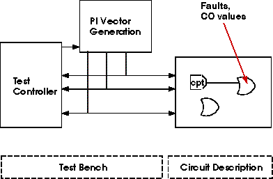
Figure 1. Adaptive Random Test Generation Environment
Electrical and Computer Engineering Department
Faculty of Engineering, Campus No. 2
University of Tehran
14399, Tehran IRAN
Tel: +98-21-800-8485; Fax: +98-21-646-1024
Email: navabi@ece.ut.ac.ir
This paper presents a VHDL test bench for random generation of test vectors for gate level structural digital circuits. Adaptive generation of test vectors is being focused here. In this approach, one of several predetermined vector generation schemes is selected based on the anticipated fault detection rate.
In some of our earlier works, we have presented VHDL models for Critical Path Tracing (CPT [1]). A circuit using these models is able to report its detected structural faults on its internal lines. We have also presented VHDL fault collapsing models [2] that are able to generate a list of distinguishable faults. The test bench being presented here assumes that a fault list is available and it selects a random test vector generation scheme in order to detect faults of such a fault list with fewer number of test vectors. Each test vector is generated based on a given signal probability (probability of a line being 1'), determining random test generation scheme. Fault detection is done by activating critical path tracing VHDL models.
The process of test generation is an adaptive one [3]. Test vectors are generated on circuit primary inputs. Depending on controllability and observability of each circuit line, calculated for a given scheme (PI signal probability), detection probability of specific line faults (sa0 or sa1) can be calculated. Fault detection probabilities for fault not yet detected are instrumental in the calculation of the anticipated fault detection rate for a given random test generation scheme. At fixed intervals during the test generation process, fault detection rate for all possible test generation schemes are calculated, and the scheme with the best rate will be selected for the next test generation interval. In addition to Critical Path Tracing and Fault collapsing VHDL models, adaptive test generation also requires VHDL models for calculating line controllability and observability, as well as VHDL models for application of test data with given signal probabilities to circuit primary inputs. Fault collapsing (FC) and controllability & observability (CO) models are used independently to generate circuit fault list and line CO values. LFSRs are used for generation of test vectors for various schemes. A test controller written in VHDL is responsible for application of data to circuit under test, preparing FC and CO information, selecting appropriate schemes, and reporting the generated tests.
In this paper we will describe the complete adaptive random test generation environment with emphasis on the techniques used for selection of test schemes. Section 2 presents the test environment and the role of the test controller. In section 3 we will describe environment for generation for fault lists and CO data. Section 4 shows the process of keeping track of undetected faults. In Section 6 we will discuss models for primary inputs for generation of specific adaptive random test scheme. Section 7 discusses algorithms for selecting best text vector generation scheme.
The implementation of adaptive random test generation requires the use of a VHDL circuit description and a VHDL test bench. The test bench applies data to the circuit, performs measurements and based on information received from the circuit decides the method for generation of the next set of vectors. The general block diagram is shown in Figure 1. The circuit description consists of instantiation of gate level components. The gates of the circuit are bound to critical path tracing VHDL models. Such models are capable of finding faults on their inputs and outputs for a given test vector. In addition to actual gate models, adaptive random test generation requires controllability and observability of all gate ports as well as the reduced fault list of the circuit. Therefore the circuit description consists of CPT gate models associated with CO and FC information.
Figure 1. Adaptive Random Test Generation Environment
Initially the test controller reads CO and FC external data and associates this data with gates of the circuit under test. Then, the test controller starts the process of test vector generation by specifying a test scheme for the PI vector generation VHDL models. As tests are generated and applied to the circuit the following will take place for each test vector applied:
Controller : Stores generated vectors,
Controller : Keeps a count of tests,
Circuit    : Performs fault simulation,
Circuit    : Marks off detected faults.
After application of n test vectors, the test controller stops the vector generation process and re-evaluates the vector generation scheme used for generation of PI test vectors. A test generation scheme determines signal probabilities of the individual PI lines. At the start, a scheme is used which causes all PI lines to have a probability of 0.5 for becoming 1', we will refer to this scheme as the 0.5 scheme.
The CO and remaining undetected faults of circuit gates help the test controller to decide which predefined test scheme to use for the next n test vectors. The test controller performs calculation for predicting how well each of the possible schemes will detect remaining faults. This calculation is based on CO information of each scheme and undetected fault list. Based on the result of this calculation, a test scheme for the next n test vectors will be selected.
In the sections that follow we will discuss the preparation of gate information, importing data into test controller, PI vector generation, fault simulation for marking off detected faults, and test scheme evaluation techniques.
As described in the previous section, evaluation of a test scheme requires controllability and observability of circuit lines to be known for each of the test schemes. This evaluation also requires a list of detectable faults to be available. This information is generated by running circuit gate level description with FC or CO VHDL models.
As depicted in Figure 2, a VHDL netlist corresponding to the circuit under test is bound to FC (fault collapsing) VHDL models to produce a collapsed fault list. The process of fault collapsing is referred to reducing an original fault list that contains sa1 and sa0 faults on all circuit nodes to a reduced fault list that only contains those faults that are not equivalent. Equivalent faults are those that cannot be distinguished on the primary outputs by application of test vectors on the primary inputs. VHDL models and format of the generated fault list are described in reference 2. Collapsed fault list is written to an external file.
 ___________
 |         |         _____________VHDL netlist _____________
 | Test    |         |                                     |
 | schemes |         |                                     |
 |_________|   ______|______                          _____|_______
    |          |           |                          |           |
    |          | Bind to   |                          | Bind to   |
    |--------> | CO models |                          | FC models |
               |___________|                          |___________|
                     |                                      |
                     |                                      |
              _______|_________                      _______|______
              |               |                      |            |
	      | Line CO       |                      | Complete   |
	      | Values, set i |                      | list of    |
              |_______________|                      | individual |
              |               |                      | faults     |
	      |   set ...     |                      |____________|
              |_______________|
              |               |
	      |	  set j       |
              |_______________|
|
Cout = 1 - (1 - Cin1) * (1-Cin2) = 0.625
Using controllability values and assuming an observability of 1 for the primary outputs, observability of each of the circuit lines can be calculated. Observability values calculated for circuit lines of Figure 3 are shown in this figure.
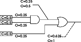
Figure 3. Controllability and Observability
The process of selecting test vector generation scheme depends on CO information for each scheme. Also as faults are detected, a list of undetected faults is necessary for selection of a proper scheme. Because this information is frequently referred to by gate models and the test controller, we have used shared variables to store CO and FC information of the circuit gates.
	TYPE faults IS ('0','1','B','N');
 	TYPE con_ob IS RECORD
    	  control : real;
    	  observe : real;
  	END RECORD;
  	TYPE con_ob_vector IS
          ARRAY ( NATURAL RANGE <> ) OF con_ob;
  	TYPE g_node;
  	TYPE g_node_ptr IS ACCESS g_node;
  	TYPE g_node IS RECORD
    	  g_type : STRING (1 TO 6);
    	  id     : POSITIVE;
    	  in_1   : faults;
    	  in_2   : faults;
    	  out_1  : faults;
    	  co_i1  : con_ob_vector (1 to repeat);
    	  co_i2  : con_ob_vector (1 to repeat);
    	  co_o1  : con_ob_vector (1 to repeat);
    	  link   : g_node_ptr; --for link list;
  	END RECORD;
|
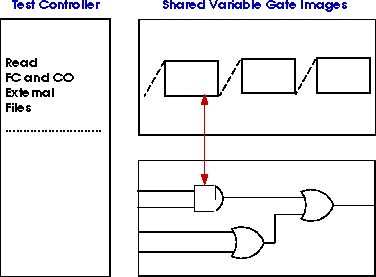
Figure 5. Shared Variable Gate Images
TYPE GATE ID [ SINGLE STUCK FAULT (SSF) LIST] AND2 ( 3 ) [ I1:sa_1 ;I2:sa_1 ;O1:sa_1,sa_0 ] . . |
NAND no. 0006 reporting : For iteration no. 0001 5.000000e-001 ; controllability of input 1 6.250000e-002 ; observability of input 1 5.000000e-001 ; controllability of input 2 6.250000e-002 ; observability of input 2 7.500000e-001 ; controllability of output 1.250000e-001 ; observability of output . . |
As test vectors are applied to the circuit under test, circuit gate models perform critical path tracing as a means of fault simulation. This mechanism enables each gate to become aware of faults on its ports that can be detected by the applied test vector. A g_node record contains faults fields for each of gate ports. The faults type, shown in Figure 4, is an enumeration type.
When FC external files are read, the faults field of a gate port will be assigned to one of the enumeration elements of the faults field. A 0' (1') signifies that a sa0 (sa1) is to be detected on that port. The value B' indicates that both sa0 and sa1 values are among the list of faults to be detected and N' indicates no fault to be detected .
A CPT gate model that becomes aware of a sa0 (sa1) fault being detected by a certain test vector changes its 0' (1') fault field value to N'. Two shared variables keep counts of original faults and detected faults. A CPT gate model is responsible for incrementing the number of detected faults when one is detected on any of its ports. The test controller uses the count shared variable for deciding on the test scheme or for stopping the test generation when a coverage is reached.
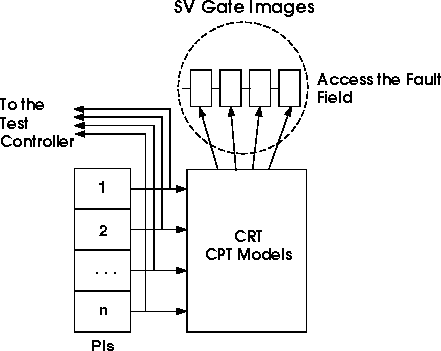
Figure 7. Test Application and Fault Mark Off
Primary input test vectors are generated by a set of parallel LFSRs. An LFSR is dedicated to generation of serial inputs for a primary input. All the PI LFSRs are coordinated by a clock signal from the test controller and a shared variable containing a fractional number representing the test generation scheme. The clock signal from the test controller signals all LFSRs to send the next data on their serial output. The LFSRs perform certain Boolean functions to make the signal probability of their outputs the same as that of the current scheme. Figure 8 shows a partial LFSR VHDL description.
PROCEDURE srpg(seed:IN qit_vector;
                              state:OUT qit_vector;
                              one_bit:OUT tit;
                              one_prob:IN real:=0.5 ) IS
    BEGIN
     -- 10: 3 0  Primitive polynomial
      state(9):=seed(0) XOR seed(3);
      state(8 DOWNTO 0):=seed(9 DOWNTO 1);
      IF one_prob = 0.25 THEN
          one_bit := seed(0) AND seed(9);
      ELSIF one_prob = 0.375 THEN
         one_bit := (seed(0) OR seed(9)) AND seed(5);
      ELSIF one_prob = 0.5 THEN
          one_bit := seed(0);
      ELSIF one_prob = 0.625 THEN
         one_bit := (seed(0) AND seed(9)) OR seed(5);
      ELSIF one_prob = 0.75 THEN
          one_bit := seed(0) OR seed(9);
      END IF;
    END srpg;
|
The test controller begins the process of random test generation with a 0.5 scheme. After generation on n test vectors (n is a user defined constant that is partially dependent on the circuit size), the test controller reads CO information of lines that still have undetected faults and makes a prediction for the rate of detection for every possible test scheme. It then selects the scheme to be used by setting the scheme shared variable to the chosen scheme (0.5, 0.25, 0.75,...). This section presents details of the selection process and evaluation techniques.
Figure 9 shows a block diagram for the selection process. As shown here a selected scheme becomes the basis of test generation for the next test interval (n). The process of selecting a scheme and adapting test pattern generation continues until a predefined fault coverage is achieved. Certain provisions for guarding against continuously changing schemes while trying to achieve a hard to reach fault coverage are put into the program.
                   ____________________________
                   |                          |
                   | Test interval := n;      |
                   | Scheme: s := 0.5;        |
                   |__________________________|
                                 |
         |---------------------->|
         |                       |
         |         ______________V_____________
         |         |                          |
         |         | Clock all PIs n times to |
         |         | Generate Test Vectors    |
         |         |__________________________|
         |                       |
         |                       |
         |                       V
         |                ______/ \_______
         |                |              |
         |                | The desired  |
         |                /  Fault       \
         |               <  Coverage ?    ><---------------|
         |                \              /           YES   |
         |                |_____   ______|                 |
         |                      \ /                        |
         |                       |                         |
         |                       |                         |
         |         ______________V_____________    ________V________
         |         |                          |    |               |
         |         | For all Schemes          |    | Output        |
         |         | Calculate Slope and      |    | Generated     |
         |         | Select Best Slope        |    | Test Vectors  |
         |         |__________________________|    |_______________|
         |                       |
         |                       |
         |-----------------------|
|
7.1 Slope Rate Calculation
To calculate this slope, we will present mathematics that lead to an expression for the exponential relation between number of random tests and fault coverage.
Detection probability of a line is determined by its controllability and observability. For a node i, the probability of a stuck-at-value fault (sa_v) being detected is that the node is observed and it can be controlled to the complement of v. The detection probabilities can be calculated as shown below:
PDsa0i = Ci * Oi
PDsa1i = (1 - Ci) * Oi
A cumulative detection probability is defined as the probability of detecting fault j given n independent trails. The equation for comulative PD for fault j is shown below:
CPDj(n) = 1 - (1 - PDj)n Given the comulative fault detection probability of a fault j, and averaging this quantity for a set of M undetected faults yields an expression that represents the fault coverage estimate as a function of n.
The above expression for fault coverage estimate represents an exponential function, shown in Figure 10. This indicates that fault detection becomes harder when fewer faults remain to be detected. The slope of this curve represents the rate of faults being detected. The expression shown below represents this rate (RFD = Rate of Fault Detection).
This expression is implemented in VHDL and is used for selecting a test scheme.

Figure 10. Fault Coverage Estimate
A test scheme is selected based on the rate of fault detection. The parameters used for this calculation are M (total number of undetected faults), PD (probability of detecting undetected faults), and n (number of tests applied).
The total number of undetected faults (M) is available in a shared variable. PD for each gate input or output and for all test schemes is available in the shared variable image record (Figure 5). The controller keeps a count of number of applied tests (n).
|
|
At the end of a test interval, the coverage impure function and the current fault coverage is compared with the desired coverage. If the desired coverage is not achieved the compute_one_prob procedure is called to predict the best test scheme in the next test interval, and sets the shared variable corresponding to the test scheme.
We have presented a test environment for adaptive test generation in VHDL. The method uses fault simulation, fault collapsing, and controllability and observability calculations, for which VHDL gate models have been developed. The test bench and other utilities used in this implementation have all been coded in VHDL. In all such implementations we have taken advantage of VHDL 93 shared variables.
The method for the selection of test schemes has been developed so that it can be implemented in VHDL. At the timing of writing of this paper, the implementation is complete, but more tests and comparisons have to be made. Running benchmarks for comparing our method with other adaptive test generation methods in part of the continued work on this project.
This implementation is part of series of projects for an all-VHDL test solution [1, 2, 3, 4, 5].